Liquidity, Money Supply and the Velocity of Money: The “Invisible Pulse” Behind Growth and Inflation
Ryan Lidder - May 25, 2026
Executive Summary
Liquidity is one of the most important macro forces behind market cycles. M2 measures the broad amount of money available in the economy, QE is one method central banks use to add liquidity and lower longer-term rates, and velocity of money determines how actively that money circulates through the real economy. The S&P 500 is influenced by all three through valuation multiples, earnings growth, interest rates and investor risk appetite.
Why Liquidity Matters
Financial markets are often explained through earnings, interest rates, inflation, valuations and investor sentiment. Those factors matter. But beneath many major market cycles sits another powerful force: liquidity.
Liquidity refers to the availability of money and credit within the financial system. When liquidity is abundant, capital tends to move more freely into businesses, real estate, bonds, private markets and public equities. When liquidity contracts, investors often become more selective, financial conditions tighten and valuation multiples can come under pressure.
Three concepts are especially important for understanding this relationship: M2 money supply, quantitative easing (QE) and the velocity of money. Together, these help explain why equity markets, including the S&P 500, often respond strongly to changes in monetary policy and financial conditions.
M2: The Amount of Money in the System
M2 money supply is a broad measure of liquid money available in the economy. It includes cash, chequing deposits, savings deposits, small time deposits and retail money market funds. FRED’s M2 series is published by the Federal Reserve and, as of March 2026, U.S. seasonally adjusted M2 was approximately $22.7 trillion.
In simple terms, M2 represents the pool of liquid purchasing power available to households, businesses and investors. When M2 is growing quickly, more money is available for spending, saving, lending and investing. When M2 slows or contracts, the financial environment often becomes less supportive.
That does not mean every new dollar in M2 flows directly into the stock market. Some money remains in bank deposits. Some is used for consumption. Some pays down debt. Some moves into bonds, real estate, private businesses or money market funds. But at the broad macro level, a larger pool of liquidity can support higher asset prices, especially when interest rates are low and investors are encouraged to seek higher returns.
QE: How Central Banks Add Liquidity
Quantitative easing, or QE, is a monetary policy tool used when central banks want to ease financial conditions beyond simply cutting short-term interest rates. Under QE, the Federal Reserve buys longer-term securities such as Treasury bonds and agency mortgage-backed securities. The goal is to lower longer-term yields, support credit markets and make broader financial conditions more accommodative.
The New York Fed describes the large-scale asset purchase programs after 2008 as a way to put downward pressure on longer-term interest rates, support mortgage markets and improve broader financial conditions.
When the Fed buys securities, it increases reserves in the banking system and removes longer-duration bonds from the market. This tends to push bond yields lower. As yields fall, investors often move further out on the risk spectrum in search of return. That portfolio rebalancing process can support corporate bonds, real estate, private assets and equities.
For the S&P 500, QE can help through two main channels: lower discount rates, which increase the present value of future earnings, and higher risk appetite, which can lead investors to pay higher valuation multiples for equities.
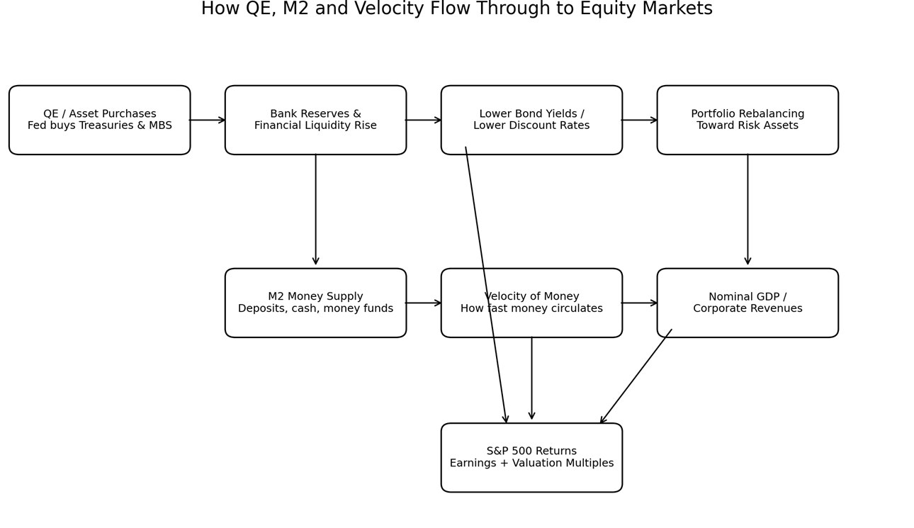
Figure 1: How QE, M2 and velocity flow through to equity markets.
The Missing Link: Velocity of Money
Money supply alone does not tell the full story. The other critical variable is velocity of money.
Velocity measures how frequently money is used to purchase goods and services. FRED defines M2 velocity as the ratio of quarterly nominal GDP to the quarterly average of M2 money stock. In plain language, it measures how often each dollar of M2 turns over in the economy.
The basic relationship is: Nominal GDP = Money Supply × Velocity. Or, stated another way: Velocity = Nominal GDP / Money Supply.
This is crucial. If the money supply increases but velocity falls, the added money may not produce as much real economic activity or inflation. It may sit in bank accounts, reserves, money market funds or financial assets. If the money supply increases and velocity rises, the money is actively circulating, which can support stronger nominal GDP, corporate revenues and earnings.
FRED reported M2 velocity at approximately 1.411 in Q1 2026, meaning each dollar of M2 was turning over a little more than once per year in relation to nominal GDP.
A useful analogy is: M2 is the amount of fuel in the tank. QE is one way of adding fuel. Velocity is how quickly the engine burns that fuel.
Why Liquidity Can Lift Asset Prices Before the Economy Accelerates
One of the most important market lessons from the post-2008 period is that liquidity can support asset prices even when the real economy remains relatively subdued.
After the Global Financial Crisis, the Federal Reserve expanded its balance sheet through multiple rounds of QE. Those policies lowered interest rates and supported financial markets. However, M2 velocity remained in a long-term downward trend.
That combination produced an important outcome: financial liquidity increased, interest rates remained low, investors moved into risk assets, equity valuations expanded, but money did not circulate through the real economy as quickly as in prior decades.
As a result, the post-2008 period was highly supportive for financial assets but did not immediately produce the kind of broad consumer price inflation many expected. A key reason was that money velocity remained weak. Liquidity flowed into markets, but the turnover of money in the real economy stayed relatively low.
Why the COVID Period Was Different
The COVID period was different because monetary stimulus was paired with very large fiscal stimulus. QE expanded the Federal Reserve’s balance sheet, but government transfers and emergency support programs also pushed money directly into household and business accounts. This caused a sharp increase in M2 during 2020 and 2021.
At first, velocity collapsed because the economy was partially shut down. People and businesses had more cash, but fewer opportunities to spend it. As the economy reopened, however, that stored liquidity began circulating more actively.
This combination, high money supply plus recovering velocity, was much more powerful than QE alone. It supported nominal GDP growth, corporate revenues, consumer demand and eventually inflation pressure.
The key distinction is QE with low velocity can inflate financial assets. QE and fiscal stimulus with rising velocity can inflate both asset prices and the real economy.
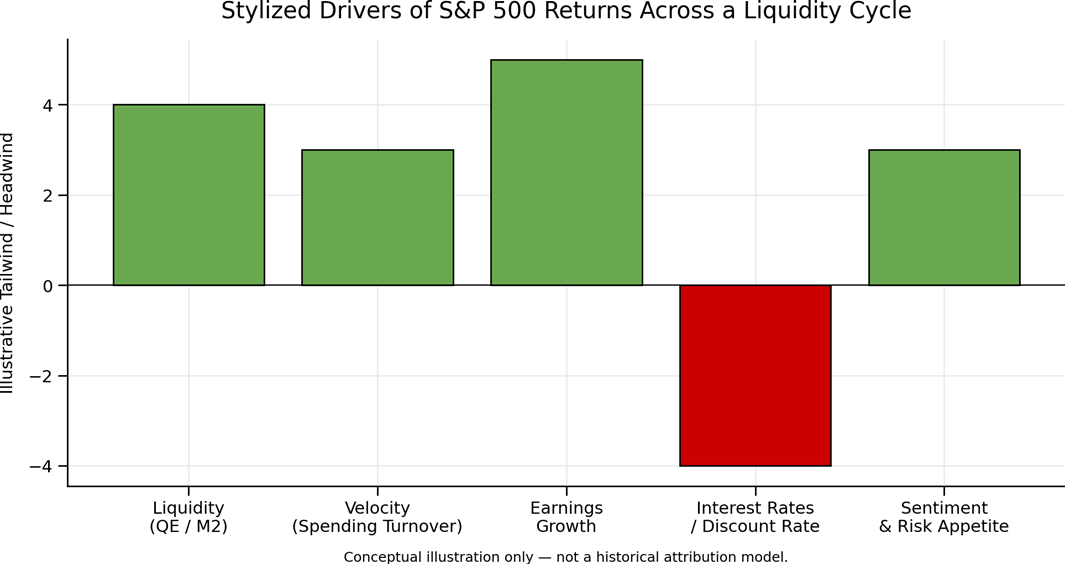
Figure 2: Stylized drivers of S&P 500 returns across a liquidity cycle. Conceptual illustration only — not a historical attribution model.
The S&P 500 Responds to Both Liquidity and Earnings
The S&P 500 is influenced by two broad forces: fundamentals and valuation. Fundamentals include revenues, profit margins, earnings and dividends. Valuation reflects the multiple investors are willing to pay for those earnings.
Liquidity affects both. When QE lowers bond yields, investors often become willing to pay more for future earnings. That supports valuation multiples. When M2 expands and velocity rises, nominal spending can increase, which may support revenues and earnings. When liquidity tightens, the opposite can happen discount rates rise, risk appetite weakens and valuation multiples may compress.
The relationship is not automatic, but the pattern is clear. Liquidity can be a major tailwind or headwind for broad equity returns.
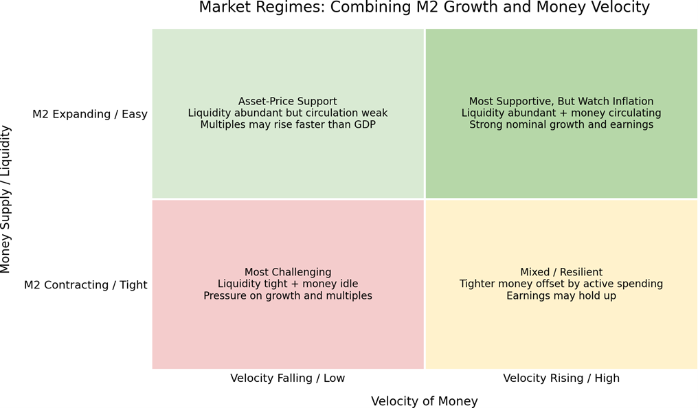
Figure 3: Market regimes combining M2 growth and money velocity
A Practical Market Regime Framework
M2 Expanding, Velocity Falling: This environment often supports financial assets more than real economic activity. Liquidity is abundant, but money is not circulating quickly. Investors may push into stocks and other risk assets because interest rates are low and alternatives are less attractive. This can lead to valuation multiple expansion.
M2 Expanding, Velocity Rising: This is generally the most powerful environment for nominal growth. Money is abundant and moving through the economy. Corporate revenues and earnings may improve. However, if inflation accelerates, interest rates may rise, which can eventually become a headwind for valuations.
M2 Contracting, Velocity Falling: This is usually the most difficult environment for risk assets. Liquidity is tightening and money is not circulating. Economic growth may slow, earnings expectations may weaken and valuation multiples may compress.
M2 Contracting, Velocity Rising: This is a mixed environment. Tighter liquidity may pressure financial assets, but rising velocity can keep nominal GDP and earnings more resilient. Markets may become more selective, rewarding companies with strong cash flows, pricing power and durable margins.
What This Means for Investors
Liquidity cycles matter. Markets tend to perform better when liquidity is expanding, financial conditions are easing and investors are encouraged to take risk. When liquidity contracts, return expectations should become more conservative.
Velocity determines whether liquidity reaches the real economy. If money supply expands but velocity remains low, the impact may show up more in asset prices than in GDP growth. If velocity rises, the impact can broaden into revenues, earnings and inflation.
Inflation changes the interpretation. Rising velocity can be positive when it reflects healthy economic activity. But if it contributes to excessive inflation, central banks may tighten policy. That can reverse the valuation benefit that liquidity initially created.
Valuation discipline matters more when liquidity slows. In a high-liquidity environment, markets often reward long-duration growth assets. In a tightening environment, investors tend to favour quality, cash flow, profitability, balance sheet strength and valuation discipline.
Bottom Line
The link between M2, QE, money velocity and S&P 500 returns can be summarized simply: M2 tells us how much money exists. QE is one way central banks add liquidity. Velocity tells us how actively that money is moving through the economy. The S&P 500 responds to both liquidity-driven valuation changes and velocity-driven earnings growth.
When liquidity is abundant, rates are low and velocity is improving, the backdrop can be supportive for equities. When liquidity is contracting, velocity is falling and rates are rising, markets often face a more challenging environment.
For clients, the simplest framing is: money supply is the fuel, QE adds fuel, velocity determines how quickly the fuel moves through the economic engine, and the stock market responds to both the amount of fuel available and how productively that fuel is being used.
Reference
- Federal Reserve Bank of St. Louis, FRED, “M2 (M2SL).”
- Federal Reserve Board, Governor Michelle W. Bowman, “The Federal Reserve’s Balance Sheet as a Monetary Policy Tool: Past Lessons and Future Considerations,” May 28, 2024.
- Federal Reserve Bank of New York, “Large-Scale Asset Purchases.”
- Federal Reserve Bank of St. Louis, FRED, “Velocity of M2 Money Stock (M2V).”
- Investopedia, “Understanding the Velocity of Money: Definition, Formula, Real-World Examples,” updated April 27, 2026.
- Federal Reserve Bank of St. Louis, FRED, “M2, Percent Change from Year Ago / H.6 Money Stock Measures.”
- Federal Reserve Bank of St. Louis, FRED, “S&P 500 / M2.”
- Congressional Research Service, “The Federal Reserve’s Balance Sheet and Quantitative Easing,” June 28, 2022.